Loading...
My first NBA model was a spreadsheet with 14 columns and a prayer. I plugged in pace, offensive rating, defensive rating, and a rudimentary rest variable, then compared my projected spread to the sportsbook’s line. It was crude, and it lost money for two months. But it taught me something critical: a bad model that forces you to quantify your opinion is worth more than a good hunch you never test. Five iterations later, that spreadsheet became a model that has been profitable four of the last five seasons.
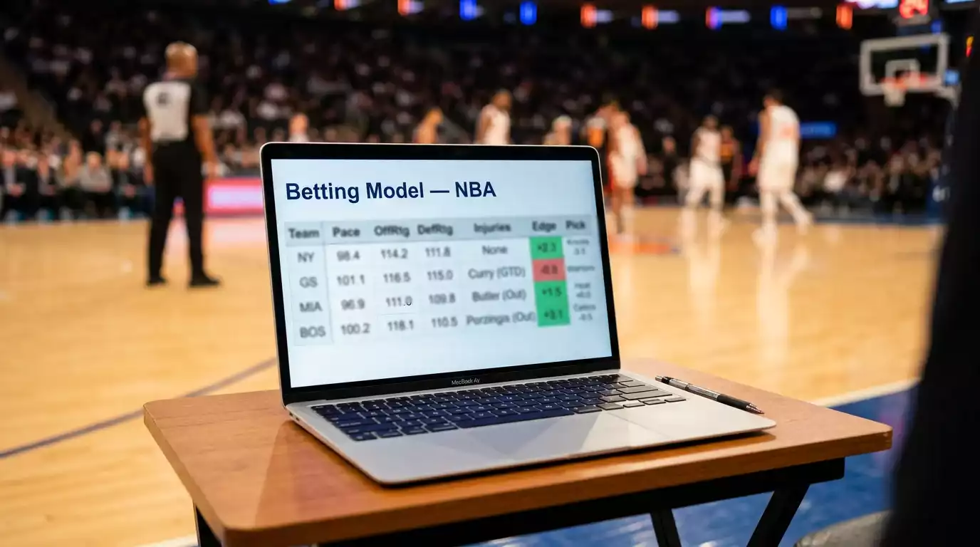
NBA betting models aren’t magic. They’re structured frameworks that convert publicly available data into probability estimates, then compare those estimates to the implied probabilities embedded in sportsbook lines. When the gap between model output and market price exceeds your threshold, you have a potential bet. When the gap is small or nonexistent, you sit out. The model removes emotion, imposes discipline, and creates a repeatable process that you can evaluate and improve over time.
Block props alone show a win rate of 69.9% on overs, three-point props hit at 63.2%, and steal props at 61.9% across more than 10,580 graded predictions this season. Those aren’t random numbers — they’re output from models that process matchup data, usage patterns, and defensive tendencies to identify systematically mispriced lines. Whether you build your own model or use publicly available tools, the underlying logic is the same: data in, probability out, compare to the market.
Key Model Inputs: Pace, Efficiency, Rest, and Matchup Data
Every NBA model, from a hobbyist spreadsheet to a professional operation, needs a core set of inputs. The quality of your model depends on which variables you include, how you weight them, and how you handle recency — recent performance matters more than season-long averages, but overweighting the last five games introduces noise.
Pace — possessions per 48 minutes — is the foundation. It determines the volume of scoring opportunities for both teams. Two teams that each average 100 possessions per game will produce a game with approximately 100 possessions (slightly adjusted for home court and game context). A team averaging 105 possessions facing a team at 95 will settle somewhere in between, weighted toward the faster team since they control tempo more aggressively. Getting the possession estimate right calibrates every other projection in the model.
Offensive and defensive efficiency — points per 100 possessions — are the next layer. Research on NBA game dynamics, including a 10-year analysis of 2,295 games, shows that roughly 19% of NBA games remain within 10 points entering the fourth quarter. That competitive balance means small edges in efficiency estimation translate directly into better spread projections. I use a rolling 15-game window for efficiency metrics, which balances recency against sample size noise.
Physical performance drops significantly across quarters, with Garcia et al. documenting an effect size of -1.27 from the first to the fourth period. Incorporating rest days, travel distance, and back-to-back status into the model accounts for this decay. A team on the second night of a road back-to-back will have suppressed fourth-quarter efficiency, which affects the projected total and the projected margin.
Matchup data adds the specificity that aggregate numbers miss. How does Team A’s pick-and-roll offense perform against Team B’s drop coverage? Is Team A’s primary scorer a wing who’ll face a lockdown defender? These variables are harder to quantify but essential for model accuracy. I code matchup adjustments as binary flags (favorable/neutral/unfavorable) rather than trying to assign precise numerical values, which reduces overfitting while still capturing the directional effect.
Machine Learning vs. Regression: Common NBA Modeling Approaches
When people hear “NBA betting algorithm,” they think machine learning, neural networks, and AI buzzwords. The reality is more boring and more practical. Most profitable NBA models use some form of regression analysis — statistical techniques that have been around for decades — because regression is interpretable, resistant to overfitting on small datasets, and easy to update mid-season.
Linear regression is the workhorse. You define your outcome variable (point spread or total), input your features (pace, efficiency, rest, matchup), and the regression assigns a coefficient to each feature that represents its weight in the final projection. The output is a projected spread that you compare to the market line. The advantage of regression is transparency: you can see exactly why the model likes a particular game and diagnose errors when it misses.
Machine learning models — random forests, gradient boosting, neural networks — handle nonlinear relationships that regression misses. They can detect interaction effects (e.g., back-to-back fatigue matters more for older rosters than younger ones) without you manually coding those interactions. The drawback is complexity. A neural network might produce slightly better predictions, but you can’t easily explain why it favors one side, which makes it harder to trust during losing streaks and harder to improve when the model underperforms.
My recommendation: start with regression. Build a model you understand completely, track its performance for a full season, and identify where it fails systematically. If it consistently misses on specific game types (divisional matchups, altitude games, post-All-Star-break fatigue), add features or switch to a more flexible algorithm for those subsets. The best model is the one you trust enough to follow during a 7-game losing streak.
Backtesting and Closing Line Value as Validation Metrics
Wayne Taylor, a marketing professor who studies the sports betting industry, has observed that states opened a can of worms with legalization and are now realizing the complexity of the market they’ve created. That complexity extends to model validation — the process of determining whether your algorithm actually works or just got lucky.
Backtesting — running your model against historical data to see how it would have performed — is the first validation step. Feed your model last season’s inputs and compare its projected spreads to the actual outcomes. Did it identify profitable sides? What was the simulated ROI? Backtesting catches obvious errors (your model loves road underdogs by 10 points, which never happens) and provides a baseline performance estimate. But it also introduces survivorship bias: you’ve already seen the outcomes, and your model may unconsciously be tuned to fit those specific results.
Closing line value (CLV) is the more rigorous validation metric. CLV measures whether you’re consistently betting lines that move in your favor after you bet them. If you bet Team A -3 and the line closes at -4, you captured a point of CLV — the market moved toward your position, confirming that your bet was on the sharp side. Tracking CLV over 200+ bets is the single best indicator of whether your model identifies genuine edges or just catches variance.
I track CLV religiously. Over the last three seasons, my average CLV has been about 0.7 points per bet. That sounds small, but it compounds into meaningful profit over volume. More importantly, CLV is predictive in ways that win rate isn’t. A bettor winning at 56% might be on an unsustainable hot streak. A bettor consistently capturing 0.5+ points of CLV is demonstrating a systematic edge that the market confirms.
No model is permanent. The NBA evolves — rule changes, pace trends, roster construction philosophies — and a model that worked in 2023 might underperform in 2026 without updates. I rebuild my feature set every offseason, test new variables, and discard ones that have lost predictive power. The algorithm isn’t the edge. The process of continuously refining the algorithm is the edge, and that process starts with understanding what you’re building and why the market leaves room for it.